Is the wind against me?
Me and my friend always complain about headwind as we bike to and from university, and this got me wondering, is the wind biased? Do I suffer from more headwind than I do tailwind?
I decided to test this hypothesis based on data historical weather data from the Open-Meteo historical weather API, which builds on the ERA5, ERA5-Land and CERRA programs which are acknowledged below:
ERA5: Generated using Copernicus Climate Change Service information 2022.

ERA5: Hersbach, H., Bell, B., Berrisford, P., Biavati, G., Horányi, A., Muñoz Sabater, J., Nicolas, J.,
Peubey, C., Radu, R., Rozum, I., Schepers, D., Simmons, A., Soci, C., Dee, D., Thépaut, J-N. (2018):
ERA5 hourly data on single levels from 1959 to present.
Copernicus Climate Change Service (C3S) Climate Data Store (CDS). (Updated daily), 10.24381/cds.adbb2d47

ERA5-Land: Muñoz Sabater, J., (2019): ERA5-Land hourly data from 1981 to present. (Accessed on daily), 10.24381/cds.e2161bac

CERRA: Schimanke S., Ridal M., Le Moigne P., Berggren L., Undén P., Randriamampianina R., Andrea U., Bazile E.,
Bertelsen A., Brousseau P., Dahlgren P., Edvinsson L., El Said A., Glinton M., Hopsch S., Isaksson L., Mladek R.,
Olsson E., Verrelle A., Wang Z.Q., (accessed on 2022-12-31), doi: '10.24381/cds.622a565a'
Effective Wind
Firstly, I construct my route to and from university as a series of latitudal and longtitudal points using this route planner applet which allows me to export it as an xml file called a gpx file. The route is seen in the graph below.
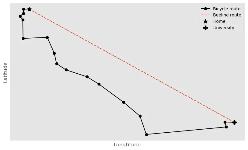
My route from home to university as longitudes and latitudes.
The wind direction and speed is a vector field, that is, a function of a vector (latitude and longitude) which produces a vector (wind speed and direction). My route is about 5 km long, and since the Open-Meteo API does not have such large resolution, the wind is the same in every point on the route. Therefore, the wind vector field is constant and is therefore conservative, since it is the gradient to a function.
Let $v_1, v_2$ be the constant wind speed in the longtitudal and latitudal directions, then we may describe the vector field $v$ as gradient of $F(x)$. $$ v = \begin{bmatrix}v_1 \newline v_2\end{bmatrix} = \begin{bmatrix} \frac{\partial F}{\partial x_1} \newline \frac{\partial F}{\partial x_1} \end{bmatrix} = \begin{bmatrix} \frac{\partial}{\partial x_1} v_1 x_1 + v_2 x_2 \newline \frac{\partial}{\partial x_1} a_1 x_1 + a_2 x_2 \end{bmatrix} $$
A conservative field has the same integral for any path taken through it. In discrete terms, this means that any sum of path segments is the same. Therefore, the Beeline route in the above plot is equivalent to the Bicycle route when it comes to calculating total amount of wind experienced.
Therefore, the route can be thought of as a single vector, one that goes from home to university in the morning and university to home in the afternoon. If we normalise this vector to 1 and perform the dot product of the wind vector, we acquire the effective wind speed experienced. This is because the route vector is a unit vector, meaning that the dot product is a vector projection of the wind speed onto the route.
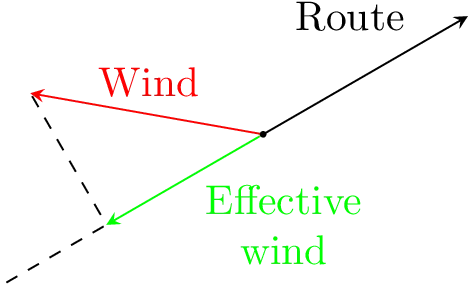
Effective wind speed i.e. the wind speed experienced en route.
If I perform the dot product on the entire data set retrieved from Open-Meteo, I obtain the effective wind speed en route for every hour of every day within the chosen time period.
I have been biking approximately the same route to the same university faculty for around 4 years, so I will examine data in the period 2019-01-01 to 2023-03-10 (YYYY-MM-DD format).
The plot below shows a histogram of the effective wind speeds in this period as given by Open-Meteo.
Since the vector is defined from home to university, a positive speed means tailwind while a negative speed means headwind. Remark that $n$ is the amount of samples, $\mu$ is the sample mean and $\sigma$ is the sample variance.
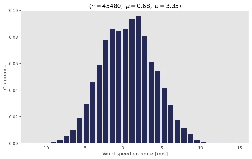
Wind speed for every hour of every day between 2019-01-01 and 2023-03-10 or 1895 days
The mean being positive is not that remarkable, as my route to university is mostly eastwards which coincides with the prevailing winds from west. This means that I will generally experience tailwind commuting to university and headwind commuting home. Still, the question remains - do I suffer quantitively more headwind than tailwind?
Limiting to commutes
To figure out if I generally experience more headwind or tailwind on my commute I have to limit the data to periods where I actually commute. In general, my commuting schedule is:
- I only commute Monday through Friday
- At 08:00 I commute to university
- At 16:00 I commute back home
Filtering these points from the data is trivial, since every point includes a timestamp. It is worth noting that the effective wind speed on the commute back home is negative as the route vector is flipped. A data set is also be constructed by adding both commutes, which is denoted the Total commute.
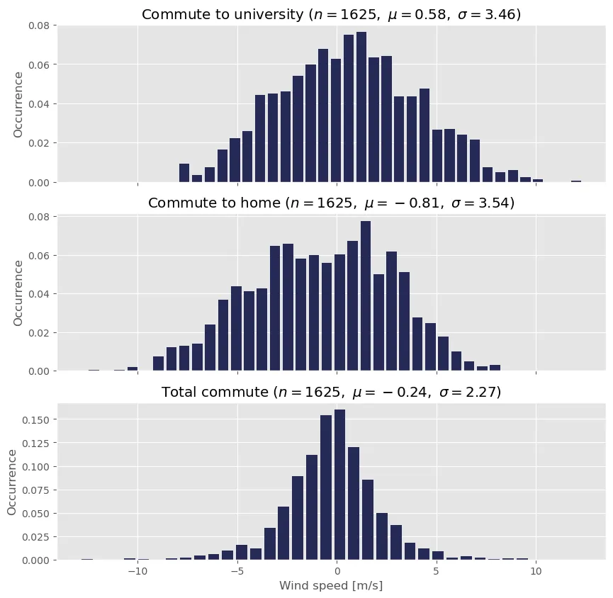
Effective wind speed for the morning commute, afternoon commute and total commute.
In general, it appears that I experience tailwind on the way to university and headwind back home, which is consistent with the prevailing west winds. Still, it appears that I suffer a little more headwind on the way home than tailwind on the way to university. Does this mean, that the wind is indeed biased?
Statistical Test
When the total commute is positive, I experience more tailwind than headwind the corresponding day; the opposite is true for a negative total commute wind speed. If the wind is not biased towards giving me more or less headwind, one would expect this total commute to tend to 0. One could argue that the mean $\mu=-0.24$ already being negative proves that I experience more headwind than tailwind. However, it is possible that the mean actually is zero and I was simply unlucky.
This is the realm of hypothesis testing, where problems like this are common. Let us assume that the distributions are normal. I propose the following null-hypothesis $H_0$ and alternative hypothesis $H_1$:
- $H_0:$ The mean of the total commute windspeeds is greater than or equal to zero
- $H_1:$ The mean of the total commute windspeeds is less than zero
Let the mean of the underlying process of total commute wind speeds be $\mu$ and the sample mean of the total commute wind speeds be $\mu_0$. The hypotheses are then expressed as:
- $H_0: \mu \geq 0$
- $H_1: \mu < 0$
Since the variance of the underlying process is unknown, this is known as an unpaired one-sided t-test. In such a test, it is assumed that a test statistic $TS$ is distributed according to a Student’s t-distribution with $n-1$ degrees of freedom $$ \begin{aligned} S^2 &= \left(\frac{\sum_i (X_i - \bar X)^2}{n-1} \right) \newline TS &= \frac{\sqrt{n}(\bar X - \mu_0)}{S} \sim t_{n-1} \end{aligned} $$ Here, $X$ are the random samples i.e. the total commute wind speeds and $\bar X$ is the sample mean. Where the test statistic lands on the distribution tells us how likely we are to see our results given our null hypothesis. That is, a more extreme $TS$ (far away from 0) makes it more likely that the mean is not zero. The plot below shows the probability density function (PDF) of the t-distribution where $\nu$ is the degrees of freedom $n$.

Student's t-distribution. Skbkekas, CC BY 3.0 <https://creativecommons.org/licenses/by/3.0>, via Wikimedia Commons
Since this is a one-sided test, we are examining how likely it is to obtain the results we’ve seen or more extreme given the null hypothesis. More extreme in this case means a more negative $TS$ as this entails a more unlikely result wrt. the null hypothesis which claims it is greater or equal to 0. The likelihood of a more extreme $TS$ for this one-sided test is the area under the distribution (the integral) from $TS$ towards $-\infty$. The value for this is given by the cumulative distribution function (CDF) which for example is defined in the Python library SciPy.
The probability of the data being distributed with a mean $\mu \geq 0$ for the given data is $p = 1.357 \cdot 10^{-5}$. This is possible but extremely unlikely, and hence we can with 99% certainty dismiss $H_0$. As such, we accept the alternative hypothesis that $\mu < 0$, that is:
We can reasonbly deduct, that me and my friend generally do suffer from more headwind than tailwind on our commutes.
Still, we cannot deduct from this test how much more headwind we experience as such a test would be significantly more difficult to construct.
 Disclaimer
This hypothesis test merely proves that me and my friend experience greater headwind speeds when commuting home than commuting to university. It does not prove that the force exerted onto our bodies due to this wind is greater on our commute home than to university.
The force from the wind is dependent on many factors and is frankly a study of its own.
Published 24. March 2023
Last modified 20. April 2023